
The 9-1 Knot

Knots and crossing numbers

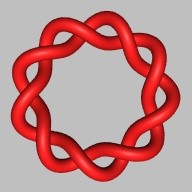
A knot is a simple, closed, non-self-intersecting curve in \(R^3\). It is natural to think of a knot as constructed from a string glued together at the ends, usually tangled in the middle.
The knot for my project is knot 9-1 in the knot atlas, which is centrosymmetric. The crossing number of the knot is 9.
It is common to use a knot diagram or 2D projection to graphically represent knots. A knot is represented by a curved line on the page. When the knot passes under itself, a gap is used at the crossing. The projection of the 9-1 knot is shown in the following picture:

Sequence of crossing switches for unknotting

There are three types of simple allowed ways to deform knot diagrams by changing the number of crossings as shown in the following picture.
The unknotting number of a knot is the minimum number of times to switch the crossing points to untie it. The 9-1 knot has the unknotting number \(4\). As shown in the following picture, the sequence of crossings \(1,3,5,7\) marked by red dashed line circles can be switched, then by using the Type II and Type I deforming methods, the knot is untied.

Coloring the knot

The 9-1 knot is colorable under the following rules for coloring a crossing
  1. all three colors are used; or
  2. only one color is used.
The tricolor effect of the 9-1 knot is shown in the following figure.

The writhe of the knot

Knots are frequently considered with orientation. That is, the strand of the knot is given one of two directions, indicated by arrows along the strand. Crossings can be either right-handed crossings (positive crossing, denoted by \(+1\) ), or left-handed crossings (negative crossing, denoted by \(-1\) ) with respect to the current orientation of a projection. In a knot with one component, reversing the orientation does not alter the handedness of its crossings.
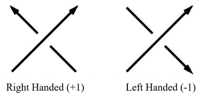
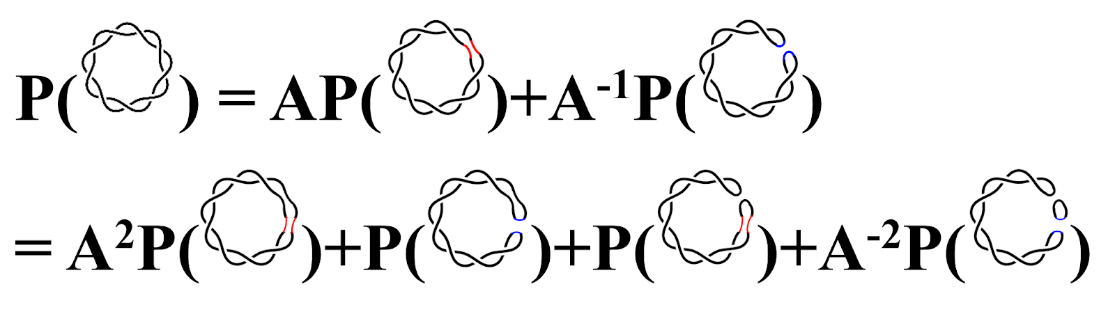
The orientation of the 9-1 knot is shown in the following figure.
The writhe of a knot is the total number of positive crossings minus the total number of negative crossings. There are 9 positive crossings in total for the 9-1 knot. The writhe of the knot is \(+9\).

Polynomial Q

The knot polynomial is a kind of knot invariants in the form of a polynomial. The Polynomial Q is calculated by splitting crossings according to the following basic rule.
The first two steps of the polynomial Q of the 9-1 knot is shown in the following picture.
In this project, I investigated the characteristics of the 9-1 knot. The final 3D print was interesting and beautiful.

Comments

Popular posts from this blog

The Approximation of a Solid of Revolution

Most math teachers I've had have been able to break down Calculus into two very broad categories: derivatives and integrals. What is truly amazing, is how much you can do with these two tools. By using integration, it is possible to approximate the shape of a 2-D function that is rotated around an axis. This solid created from the rotation is known as a solid of revolution. To explain this concept, we will take a look at the region bounded by the two functions: \[ f(x) = 2^{.25x} - 1 \] and \[ g(x) = e^{.25x} - 1 \] bounded at the line y = 1. This region is meant to represent a cross section of a small bowl. While it may not perfectly represent this practical object, the approximation will be quite textured, and will provide insight into how the process works. The region bounded by the two functions can be rotated around the y-axis to create a fully solid object. This is easy enough to talk about, but what exactly does this new solid look like? Is

Area under a region

  If you want to find the area under a region, you can draw rectangles and add the area of the rectangles together to find an aproximation. If you want to find the exact area, you use an integral bounded by the region. But what about when we introduce a 3rd plane? How do we aproximate the volume under a region when we consider all three planes? The concept is very similar. To aproximate the volume, we use rectangles but add the element of height and sum the rectangles volumes. For the actual volume, we use a double integral (using Fubini's Theorem) bounded by the region. Consider the region contained in the intersection of \[y=x^\frac{1}{2}\] \(and\) \[y=x^3.\] We are going to aproximate and find the actual volume of this region under the function \[f(x,y)=xy.\] We're going to find the aproximated area using squares, so let's zoom in a little bit until we have a 5x5 area for a total of 25 squares to work with. Do

Come visit the quadric surfaces!

 They are in the display case.  The ruled surfaces will be joining them soon!