Introduction
In mathematics, a knot is simply a closed loop. The simplest version of this is the unknot, which is a just a closed circle (imagine a ponytail holder). Knots, however, quickly become more complicated than this more basic example. This post will examine a particular knot (knot 10-84) and a few of its knot invariants.
Crossing Number
Knots are often defined by their crossing number, which is the number of times the knot’s strands cross each other. As indicated in its name, knot 10-84 is a 10 crossing knot. In order to visualize the knot, we can look at its knot projection, in which the knot is represented by a line segment broken only at its undercrossings:

Tricolorability
Now that we’ve looked at knot crossings, we will examine a potential property of knots: tricolorability. In order to understand tricolorability, it is first important to know that one strand of a knot is defined as an unbroken line segment in the knot projection. With this in mind, a knot is tricolorable when each strand can be assigned a color so that for every crossing the strands that meet there are either 1) all the same color, or 2) three separate colors. Additionally, the strands of the knot cannot all be given the same color.
A knot coloring was attempted on knot 10-84 by beginning at the upper right crossing and coloring all the strands meeting there blue. From there, a coloring could be achieved that respected the rules of tricolorability. Therefore, knot 10-84 is tricolorable.
Unknotting Number
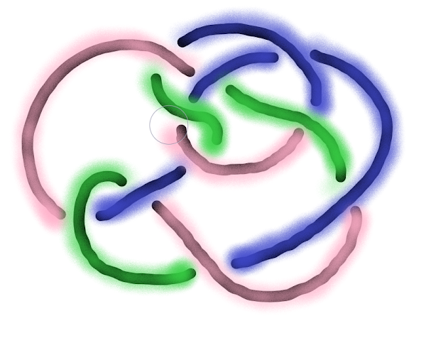
The unknotting number of a knot is the least number of crossings that need to be switched in order to turn a knot into the unknot. It is difficult to find the exact knotting number because doing so requires testing many different crossing switches. However, we will demonstrate here that our knot can be “unknotted” with three switches. The switched crossings are circled in gray in the image below:

This means that 3 is an upper bound on our unknotting number. In order to prove that this was the actual unknotting number we would need to show that changing any 1 or 2 crossings would not unknot our knot. This would be time-consuming and thus we will not prove it (however, just by looking at the knot we can hypothesize that an unknotting may not be possible with only 2 or less switches).
Writhe
Writhe is another property of a knot that is achieved by assigning numerical values to the crossings. This is achieved by first assigning the knot an orientation- in other words, imagine the knot strand is a racetrack on which cars can travel in only one direction. Each crossing is assigned either +1 or -1 based on which orientation the crossings form:

The writhe of knot 10-84 was calculated by assigning it the orientation indicated by the yellow arrows. Then, the value of each crossing was determined as is indicated in the image. To calculate the writhe, the values of each of these crossings were added. As a result, the write of knot 10-84 was determined to be -4.

Knot Polynomial
The knot polynomial is a more complicated invariant of a knot to calculate, and thus will not be done in full. The polynomial is calculated by splitting crossings according to the following rules:

We will perform two crossing splits on knot 10-84. The crossing to split on was chosen arbitrarily. The change in the knot due to the first split is indicated in red. These two polynomials were each split one more time. The changes to the knot for the first polynomial are indicated in blue, while those for the second are indicated in green:

Next, we simplify the polynomial:

This knot has many crossings, so it would be a rather long process to fully reduce them. For this reason, we will stop here. The final step is to calculate the polynomial Q using the writhe calculated previously. This gives us the following equation for the knot polynomial \( Q \):

Conclusion
Now that we’ve found some of the invariants of knot 10-84, you’ve hopefully learned a little about knot theory and can find these invariants for other knots!
Author: Sarah Bombrys
Comments
Post a Comment